Estimating sea trout smolt migration risks

I’m involved with a project aiming to understand brown trout (Salmo trutta L.) movements in freshwater and estuarine environments.

Here, I want to share the methods we used to estimate the risks to brown trout when they migrate as sea trout smolts.

But first a little background.

Background

Brown trout are funny fish.

Some spend their entire lives in freshwater, e.g., a river, and are known as brown trout. Others migrate to marine waters, e.g., an estuary or sea, and are known as sea trout.

Sea trout return to freshwater a lot larger than brown trout, after feasting on the abundant food available in marine waters, and are able to produce more eggs. Brown trout might be smaller but they don’t run the risk of being eaten by any of the abundant marine predators.

Clearly, there is a fitness trade-off between getting big & producing more eggs (maximise your potential reproduction) and avoiding being eaten by any one of the abundant marine predators (maximise your potential survival to reproduction).

The decision to migrate is not, however, black and white. Finnock are brown trout that use estuaries and transitional waters for only short periods, e.g., a couple of months, presumably to feed.

So which strategy is best: brown trout, finnock or sea trout?

To study this question, we estimated the risk to sea trout of migrating through fresh, transitional and estuarine waters.

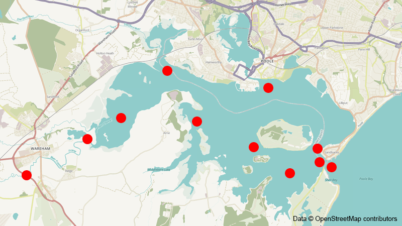
To estimate these risks, we acoustically tagged a sample of migrating sea trout smolts who’s migration pathways were recorded at listening receivers located in the different zones (Figure 1).

Location of listening receivers in Poole Harbour. Red dots represent approximate detection range of the receivers.

Analysis methods

Acoustic tracking data has the problem that detection is imperfect; we do not always detect a passing tag and so we don’t know if (i) the tag didn’t pass or (ii) whether it passed but was not detected.

This problem can and should be addressed statistically.

To estimate the risks to sea trout smolt of migrating through different zones, we used Bayesian State Space models (wikipedia: State-space representation).

I was reassured that others have used BSSMs in this context: Oliviez Gimenez’s paper explains clearly the theory of BSSMs for marked individuals and Chris Holbrook’s paper was an illustrative example of BSSM implementation for acoustically tagged lamprey.

In essence, BSSM estimates jointly the probability that a tag is detected at a particular location and the probability that it made the transition to that location successfully.

In our study, we assumed that all individuals shared the same detection and transition probabilities, i.e., that physical or behavioural differences between individuals were unimportant, and that individuals travelled independently.

We could therefore use the simple Cormack, Jolly & Seber (CJS) model given by:

\[ Y_t|X_t \sim Binomial(X_t − u_t, p_t) \]

\[ X_{t+1}|X_t \sim Binomial(X_t, \phi_t) + u_{t+1} \]

where \(X_t\) is the total number of survivors from time \(t\), which includes \(u_t\) that is the number of newly marked individuals at time \(t\), \(Y_t\) is the total number of previously marked individuals encountered at time \(t\), \(p_t\) is the probability of detecting a tagged individual at time \(t\) (\(t = 2, ..., T\)) and \(\phi_t\) is the probability that a tagged individual transitions to time \(t + 1\) given that it is alive at time \(t\) (\(t = 1, ..., T − 1\)).

This formulation separates the nuisance parameters (the detection probabilities, \(p_t\)) from the parameters of interest (the transition probabilities, \(\phi_t\)) because the latter are found only in the second or “state” equation.

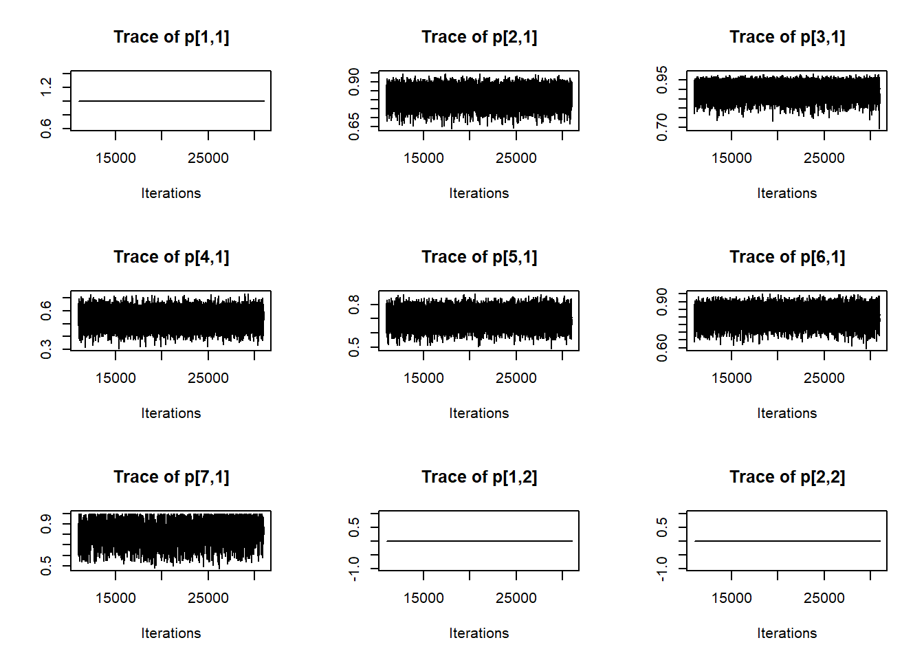
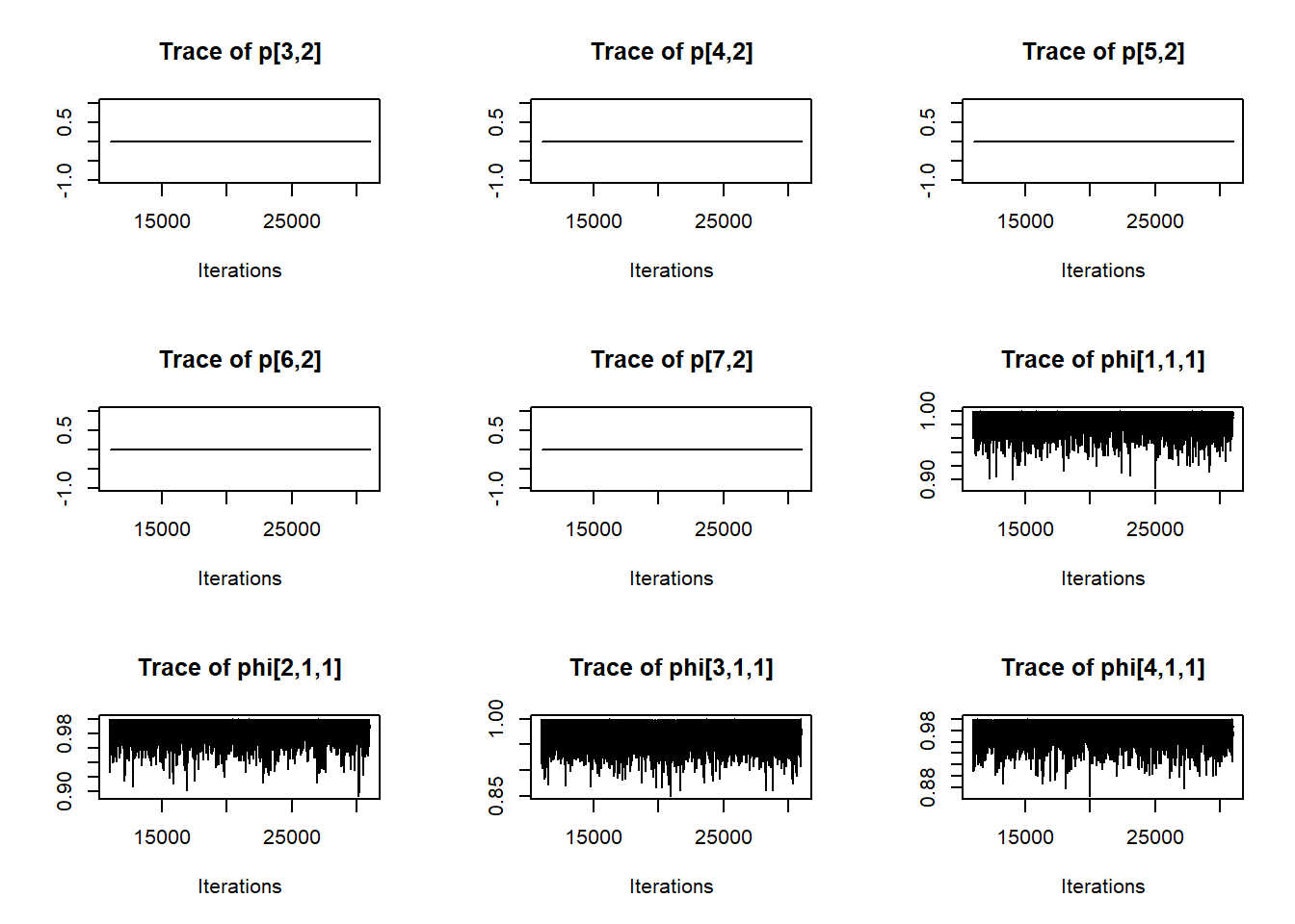
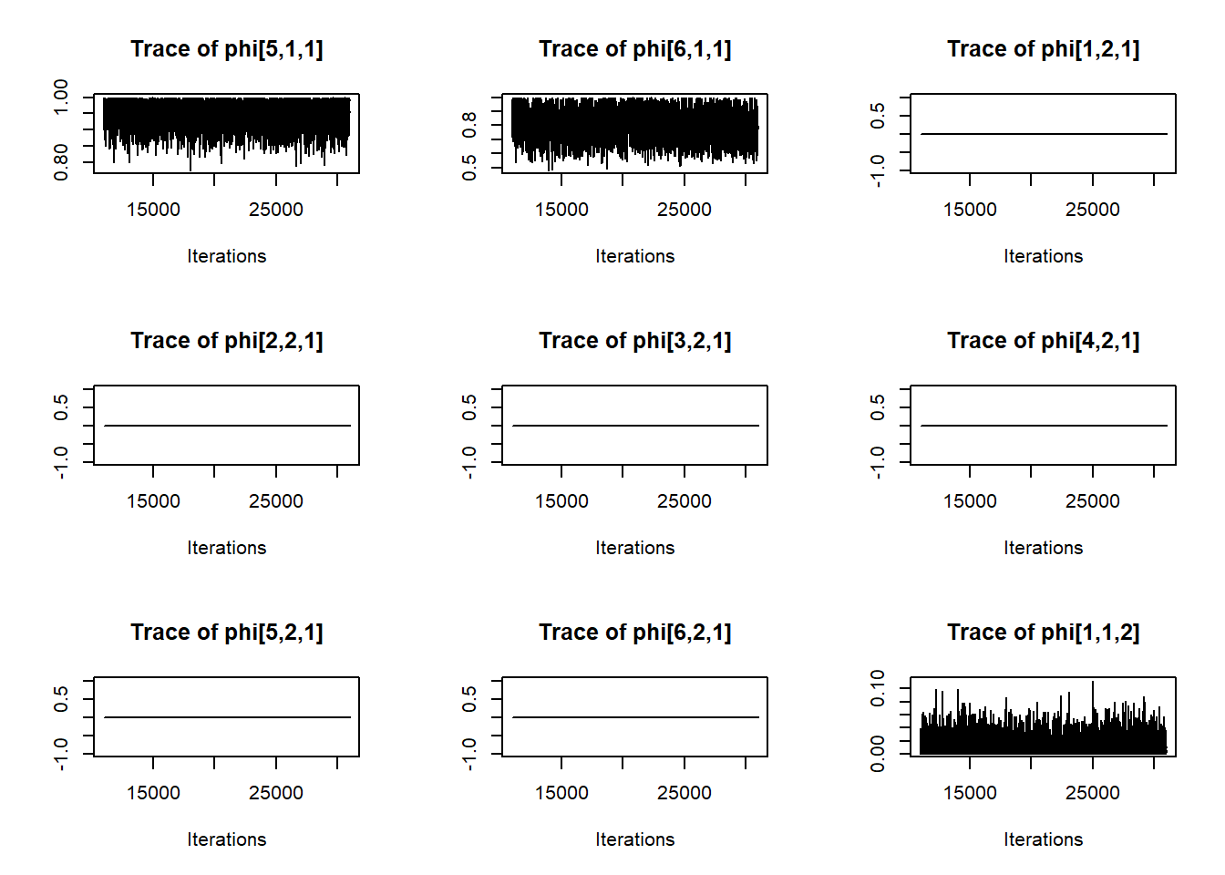
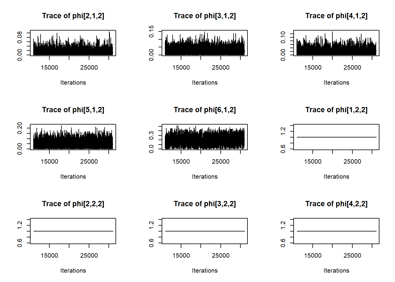
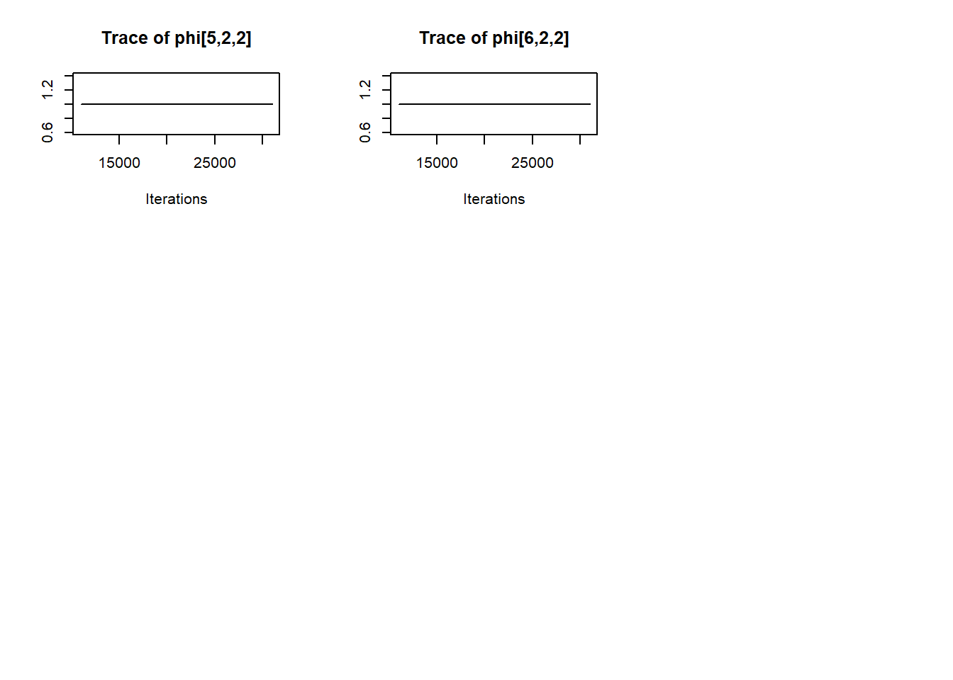
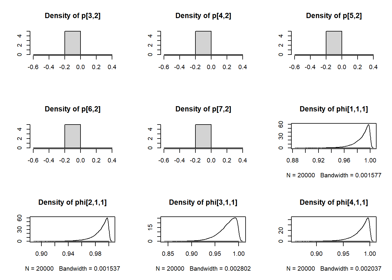
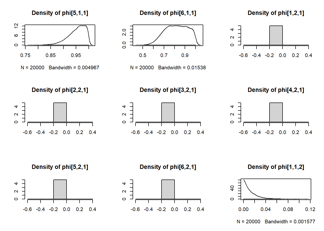
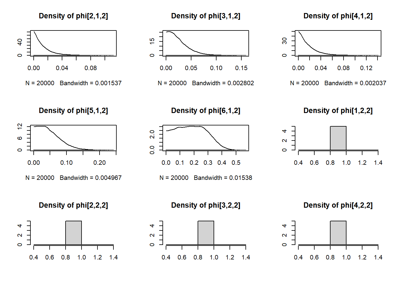
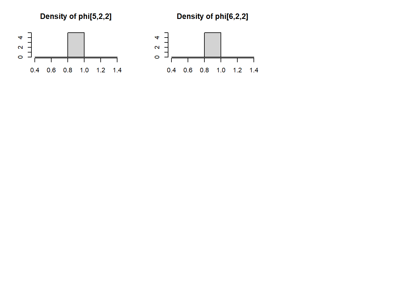
Using this model, we estimated values of \(p_t\) and \(\phi_t\) using the Monte Carlo Markov Chain (MCMC) method in JAGS. JAGS uses Gibbs sampling to explore the joint probability distribution of \(p_t\) and \(\phi_t\). Through an iterative process, weakly informative \(Beta(1, 1)\) prior distributions on \(p_t\) and \(\phi_t\) were updated with increasingly credible values until, after sufficient iterations, the best estimated values of \(p_t\) and \(\phi_t\) were taken to be the median of their posterior distributions.

We ran JAGS from within R using functions from package dclone. We ran three MCMC chains for 30,000 iterations, of which we discarded the first 10,000 as burnin.

R code to run an example BSSM is as follows:

The JAGS model file for the example might be BSSM.jags:

# simulate data
receivor_efficiencies <- c('r1' = 0.8, 'r2' = 0.9, 'r3' = 0.6, 'r4' = 0.7, 'r5' = 0.7, 'r6' = 0.7)
n_fish <- 77
ch_m <- matrix(NA, ncol = length(receivor_efficiencies), nrow = n_fish)
for(i in 1:length(receivor_efficiencies)){
    ch_m[, i] <- sample(c(0, 1), n_fish, TRUE, c((1 - receivor_efficiencies[i]), receivor_efficiencies[i]))
}
ch_m <- data.frame('release' = 1, ch_m)
colnames(ch_m)[-1] <- names(receivor_efficiencies)

# create state and observation matrices
sm <- ch_m
sm[sm == '0'] <- NA
om <- ch_m

# prep data
d <- list('sm' = sm,
          'om' = om,
          'N' = n_fish,
          'T' = ncol(ch_m))

# load libraries
library(dclone)

Loading required package: coda

Loading required package: parallel

Loading required package: Matrix

dclone 2.3-0     2019-03-21

library(rjags)

Linked to JAGS 4.3.1

Loaded modules: basemod,bugs

# name of model file
mf <- function() {

  # define likelihoods
  for(i in 1:N){
    for(t in 2:T){

      # state model
      sm[i, t] ~ dcat(phi[t - 1, sm[i, t - 1], ])

      # observation model
      om[i, t] ~ dbern(p[t, sm[i, t]])

    }
  }

  # detection probability priors and constraints

  # release
  p[1, 1] <- 1 # always observed at release
  p[1, 2] <- 0

  # r1
  p[2, 1] ~ dbeta(1, 1) # flat prior
  p[2, 2] <- 0

  # r2
  p[3, 1] ~ dbeta(1, 1) # flat prior
  p[3, 2] <- 0

  # r3
  p[4, 1] ~ dbeta(1, 1) # flat prior
  p[4, 2] <- 0

  # r4
  p[5, 1] ~ dbeta(1, 1) # flat prior
  p[5, 2] <- 0

  # r5
  p[6, 1] ~ dbeta(1, 1) # flat prior
  p[6, 2] <- 0

  # r6
  p[7, 1] ~ dbeta(1, 1) # flat prior
  p[7, 2] <- 0

  # transition probability priors and constraints

  # 1st transition
  phi[1, 1, 1] ~ dbeta(1, 1)
  phi[1, 1, 2] <- 1 - phi[1, 1, 1]
  phi[1, 2, 1] <- 0
  phi[1, 2, 2] <- 1

  # 2nd transition
  phi[2, 1, 1] ~ dbeta(1, 1)
  phi[2, 1, 2] <- 1 - phi[2, 1, 1]
  phi[2, 2, 1] <- 0
  phi[2, 2, 2] <- 1

  # 3rd transition
  phi[3, 1, 1] ~ dbeta(1, 1)
  phi[3, 1, 2] <- 1 - phi[3, 1, 1]
  phi[3, 2, 1] <- 0
  phi[3, 2, 2] <- 1

  # 4th transition
  phi[4, 1, 1] ~ dbeta(1, 1)
  phi[4, 1, 2] <- 1 - phi[4, 1, 1]
  phi[4, 2, 1] <- 0
  phi[4, 2, 2] <- 1

  # 5th transition
  phi[5, 1, 1] ~ dbeta(1, 1)
  phi[5, 1, 2] <- 1 - phi[5, 1, 1]
  phi[5, 2, 1] <- 0
  phi[5, 2, 2] <- 1

  # 6th transition
  phi[6, 1, 1] ~ dbeta(1, 1)
  phi[6, 1, 2] <- 1 - phi[6, 1, 1]
  phi[6, 2, 1] <- 0
  phi[6, 2, 2] <- 1

}

# parameters to monitor
p <- c('p', 'phi')

# initialise model
m <- jagsModel(mf, data = d, n.chains = 1, n.adapt = 1000, quiet = FALSE)

Registered S3 method overwritten by 'R2WinBUGS':
  method            from  
  as.mcmc.list.bugs dclone

Compiling model graph
   Resolving undeclared variables
   Allocating nodes
Graph information:
   Observed stochastic nodes: 800
   Unobserved stochastic nodes: 136
   Total graph size: 1331

Initializing model

update(m, n.iter = 10000)

# coda samples
s <- codaSamples(m, p, n.iter = 20000)

# plot traces
plot(s, trace = TRUE, density = FALSE)

# plot densities
plot(s, trace = FALSE, density = TRUE)

# summary
s.tab <- summary(s)
print(s.tab$statistics, digits = 3)

             Mean     SD Naive SE Time-series SE
p[1,1]     1.0000 0.0000 0.00e+00       0.000000
p[2,1]     0.8226 0.0424 3.00e-04       0.000295
p[3,1]     0.8989 0.0336 2.37e-04       0.000237
p[4,1]     0.5384 0.0571 4.04e-04       0.000404
p[5,1]     0.7078 0.0523 3.70e-04       0.000403
p[6,1]     0.8134 0.0488 3.45e-04       0.000550
p[7,1]     0.8130 0.1059 7.49e-04       0.003669
p[1,2]     0.0000 0.0000 0.00e+00       0.000000
p[2,2]     0.0000 0.0000 0.00e+00       0.000000
p[3,2]     0.0000 0.0000 0.00e+00       0.000000
p[4,2]     0.0000 0.0000 0.00e+00       0.000000
p[5,2]     0.0000 0.0000 0.00e+00       0.000000
p[6,2]     0.0000 0.0000 0.00e+00       0.000000
p[7,2]     0.0000 0.0000 0.00e+00       0.000000
phi[1,1,1] 0.9872 0.0126 8.93e-05       0.000211
phi[2,1,1] 0.9872 0.0125 8.87e-05       0.000211
phi[3,1,1] 0.9749 0.0201 1.42e-04       0.000332
phi[4,1,1] 0.9829 0.0162 1.14e-04       0.000273
phi[5,1,1] 0.9525 0.0340 2.40e-04       0.000671
phi[6,1,1] 0.8180 0.1051 7.44e-04       0.003848
phi[1,2,1] 0.0000 0.0000 0.00e+00       0.000000
phi[2,2,1] 0.0000 0.0000 0.00e+00       0.000000
phi[3,2,1] 0.0000 0.0000 0.00e+00       0.000000
phi[4,2,1] 0.0000 0.0000 0.00e+00       0.000000
phi[5,2,1] 0.0000 0.0000 0.00e+00       0.000000
phi[6,2,1] 0.0000 0.0000 0.00e+00       0.000000
phi[1,1,2] 0.0128 0.0126 8.93e-05       0.000211
phi[2,1,2] 0.0128 0.0125 8.87e-05       0.000211
phi[3,1,2] 0.0251 0.0201 1.42e-04       0.000332
phi[4,1,2] 0.0171 0.0162 1.14e-04       0.000273
phi[5,1,2] 0.0475 0.0340 2.40e-04       0.000671
phi[6,1,2] 0.1820 0.1051 7.44e-04       0.003848
phi[1,2,2] 1.0000 0.0000 0.00e+00       0.000000
phi[2,2,2] 1.0000 0.0000 0.00e+00       0.000000
phi[3,2,2] 1.0000 0.0000 0.00e+00       0.000000
phi[4,2,2] 1.0000 0.0000 0.00e+00       0.000000
phi[5,2,2] 1.0000 0.0000 0.00e+00       0.000000
phi[6,2,2] 1.0000 0.0000 0.00e+00       0.000000

where d is a list of data passed to JAGS that includes:

• \(N\) = number of individuals
• \(T\) = number of occasions
• \(sm[i, t]\) = true state matrix
• \(om[i, t]\) = observation matrix

where \(i\) is individual and \(t\) is occasion.

Our model ran without problems and the results were intuitive and as expected. We feel that this procedure worked well for us.

You will be able to read about the results in a future post.

In the meantime, use the code above to run an example BSSM and contact me if you have any problems.

Reuse

Citation

BibTeX citation:

@online{d. gregory2016,
  author = {D. Gregory, Stephen},
  title = {Estimating Sea Trout Smolt Migration Risks},
  date = {2016-01-28},
  url = {https://stephendavidgregory.github.io/posts/holbrook},
  langid = {en}
}

For attribution, please cite this work as:

D. Gregory, Stephen. 2016. “Estimating Sea Trout Smolt Migration Risks.” January 28, 2016. https://stephendavidgregory.github.io/posts/holbrook.