
What is an ordered factor?
Why might we use them?
And what are the implications of using ordered factors in statistical analysis?
If you’d like my views on these questions, then read on…
Background
What is an ordered factor?
An ordered factor is a categorical variable whose levels have a meaningful order. In the oven knob picture above, there are 4 levels: ‘OFF’, ‘LOW’, ‘MED’ and ‘HIGH’ and these should be ordered as ‘OFF < LOW < MED < HIGH’.
Why might we use them?
We often choose to use an ordered factor when it is difficult to put our variable on a meaningful continuous scale, i.e., from \(-\infty\) to \(+\infty\) where all numbers are real, e.g., not an integer or a qualitative representation of a real number, which would be a category.
Sometimes, we choose to use an ordered factor because we don’t have the equipment required to measure a variable on a continuous scale, e.g., river flow might be classified on a ordinal scale of ‘1 < 2 < 3 < 4 < 5’, which has 5 levels. This is not, however, a continuous variable.
And what are the implications of using ordered factors in statistical analysis?
When we choose to classify a continuous variable on an ordinal scale, i.e., treat the variable as a ordered factor, then we should be aware of the statistical implications for doing so. In the situation that we have a small sample size, i.e., a small number of cases, then we will likely have only few residual degrees of freedom to assess the ‘statistical significance’ of our statistical model. This is because we can only assess the ‘statistical significance’ of an ordered factor by fitting it as a polynomial term with the degree equal to the number of levels - 1. In our river flow example, the effect of river flow x on our response variable y is assessed by fitting the polynomial contrasts x^1, x^2, x^3 and x^4 (but not x^5 because one level has to be retained as the contrast level, hence the polynomial term has number of levels - 1 degrees).
In what follows, I will try to illustrate these points using simulated data in R. I present all the code so that the interested reader can run the analyses for themselves.
Statistical analysis of an ordered factor
Let’s begin by simulating some data for the multiple regression
\[y \sim \alpha + \beta_1 x_1 + \beta_2 x_2\]
In this example, \(x_1\) might be water temperature and \(x_2\) might be river flow, both recorded on their (theoretically) continuous scale \(-\infty < 0 < +\infty\). (In actual fact, river flow would be a Gamma variate because it can not be less than zero.)
Once we have simulated the data, let us fit the generating model back to the simulated data to show that we have done it correctly, and then plot the partial (or marginal) effects of each explanatory variable (Figure 1).
# load libraries
require(effects)

# simulate data; generating values
N <- 1000
a <- 5
b1 <- 5
b2 <- 3
x1 <- rnorm(N)
x2 <- rnorm(N)
sigma <- 1
epsilon <- rnorm(N, 0, sigma)
y <- a + (b1 * x1) + (b2 * x2) + epsilon

# fit lm()
lm_fit <- summary(lm(y ~ x1 + x2))

# print coefs; note they are similar to the generating values
round(lm_fit$coef, 3)
## Estimate Std. Error t value Pr(>|t|)
## (Intercept) 5.031 0.031 163.066 0
## x1 5.023 0.031 161.188 0
## x2 3.052 0.031 100.010 0# print sigma; note it is similar to its generating value
round(lm_fit$sigma, 3)## [1] 0.975# plot
foo <- lm(y ~ x1 + x2)
fii <- allEffects(mod = foo, default.levels = 50)
plot(fii)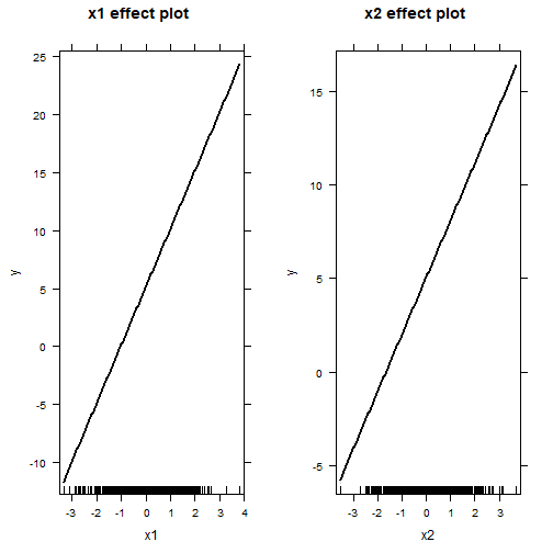
Now, what would happen if \(x_2\) had been recorded on the ordinal scale \(1 < 2 < 3 < 4 < 5\)?
# discretize x2
nLevels <- 5
x2d <- cut(x = x2, breaks = nLevels, labels = 1:5, ordered_result = TRUE)
str(x2d) # ordered factor with nLevels = 5 recorded levels
## Ord.factor w/ 5 levels "1"<"2"<"3"<"4"<..: 3 3 2 3 3 3 3 3 4 4 ...# fit discretized lm() with linear effect of x2d (coef name is x2d.L)
lm_fit_d <- summary(lm(y ~ x1 + x2d))
# "x2d.L" is significant linear effect
# note that lm() estimates nLevels - 1 (in this case, 5 - 1 = 4) coefs for the effect of x2d
round(lm_fit_d$coef, 3)## Estimate Std. Error t value Pr(>|t|)
## (Intercept) 5.491 0.111 49.650 0.000
## x1 4.978 0.049 101.562 0.000
## x2d.L 11.975 0.338 35.457 0.000
## x2d.Q 0.436 0.288 1.516 0.130
## x2d.C 0.020 0.191 0.105 0.916
## x2d^4 0.011 0.106 0.101 0.919round(lm_fit_d$sigma, 3)## [1] 1.531# plot
foo <- lm(y ~ x1 + x2d)
fii <- allEffects(mod = foo, default.levels = 50)
plot(fii)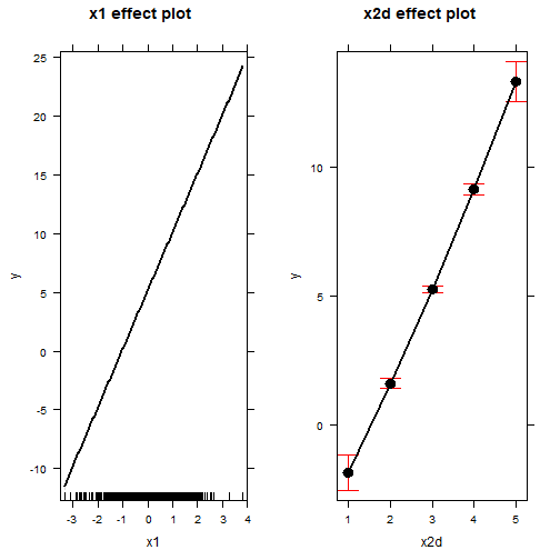
From the partial effect plots, we see that the influence of \(x_1\) and \(x_2\) on \(y\) are very similar whether \(x_2\) is treated as a continuous variable or an ordered factor.
Note, however, that the statistical model in which \(x_2\) is treated as an ordered factor has three additional coefficient estimates, representing the polynomial contrasts \(x_2^2\), \(x_2^3\) and \(x_2^4\). And the partial effect plot of \(x_2\) (x2d) on \(y\) is represented as a set of contrasts.
Note also, however, that our estimate of x2d.L (11.975 rather than 3) and sigma (1.531 rather than 1) is poor, reflecting the fact that we have not captured the true effect of \(x_2\) on \(y\) by treating the continuous variable \(x_2\) as an ordered factor.
A more correct and flexible illustration
To overcome the problem of treating the continuous variable \(x_2\) as an ordered factor, let us generate data for an example in which \(x_2\) is actually measured as an ordered factor.
Also, let us define sigLevel as the level of the ordered factor \(x_2\) that statistically influences \(y\).
# set the level at which x2 has a significant effect on y
sigLevel <- 1 # a linear effect of x_2 on y, i.e., the significant polynomial contrast is x^1

# simulate data
N <- 1000
nLevels <- 5
a <- 5
b1 <- 5
b2 <- rep(0, nLevels - 1) # nLevels - 1 contrasts; level nLevel set as contrast
b2[sigLevel] <- 3
x1 <- rnorm(N)
x2 <- gl(n = nLevels, k = N / nLevels, ordered = TRUE)
Xmat <- model.matrix(~ x1 + x2)
bvec <- c(a, b1, b2)
lp <- Xmat %*% bvec
sigma <- 1
epsilon <- rnorm(N, 0, sigma)
y <- as.numeric(lp + epsilon)

# fit lm()
lm_fit_d <- summary(lm(y ~ x1 + x2))
round(lm_fit_d$coef, 3)
## Estimate Std. Error t value Pr(>|t|)
## (Intercept) 5.006 0.032 157.573 0.000
## x1 5.000 0.031 161.650 0.000
## x2.L 3.040 0.071 42.901 0.000
## x2.Q -0.039 0.071 -0.546 0.585
## x2.C 0.048 0.071 0.673 0.501
## x2^4 -0.049 0.071 -0.696 0.487round(lm_fit_d$sigma, 3)## [1] 1.002# plot
foo <- lm(y ~ x1 + x2)
fii <- allEffects(mod = foo, default.levels = 50)
plot(fii)
That is better: the estimated coefficients for a, b1 and b2[sigLevel] and sigma are close to their generating values, and the plot shows a linear effect of \(x_2\) on \(y\).
We can change sigLevel so that the effect of \(x_2\) on \(y\) takes a different shape, e.g., a quadratic effect represented by the statistically significant polynomial contrast x^2, as follows:
# what about a quadratic effect of x2 on y
sigLevel <- 2 # a quadratic effect of x_2 on y, i.e., the significant polynomial contrast is x^2

# simulate data
N <- 1000
nLevels <- 5
a <- 5
b1 <- 5
b2 <- rep(0, nLevels - 1) # nLevels - 1 contrasts; level nLevel set as contrast
b2[sigLevel] <- 3
x1 <- rnorm(N)
x2 <- gl(n = nLevels, k = N / nLevels, ordered = TRUE)
Xmat <- model.matrix(~ x1 + x2)
bvec <- c(a, b1, b2)
lp <- Xmat %*% bvec
sigma <- 1
epsilon <- rnorm(N, 0, sigma)
y <- as.numeric(lp + epsilon)

# fit lm()
lm_fit_d <- summary(lm(y ~ x1 + x2))
round(lm_fit_d$coef, 3)
## Estimate Std. Error t value Pr(>|t|)
## (Intercept) 5.003 0.031 163.497 0.000
## x1 5.007 0.029 170.784 0.000
## x2.L -0.148 0.068 -2.161 0.031
## x2.Q 2.974 0.068 43.470 0.000
## x2.C 0.002 0.068 0.031 0.975
## x2^4 -0.057 0.068 -0.831 0.406round(lm_fit_d$sigma, 3)## [1] 0.967# plot
foo <- lm(y ~ x1 + x2)
fii <- allEffects(mod = foo, default.levels = 50)
plot(fii)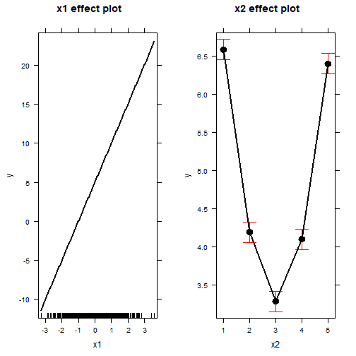
Again, note that the coefficient and sigma estimates are close to their generating values: success!
The problem of sample size…
And what are the implications of using ordered factors in statistical analysis?
In the background, I mentioned that the implications for choosing to use an ordered factor in place of a continuous variable will be particularly important when the sample size (or number of cases) is low.
This is because any statistical analysis of an ordered factor will require several contrasts (specifically, number of levels - 1 contrasts) and that those degrees of freedom are no longer “free” to assess the statistical significance of the model. This becomes particularly problematic when the number of cases is low, as illustrated for the simple linear effect of ordered factor \(x_2\) on \(y\) simulated here…
# what about a quadratic effect of x2 on y
sigLevel <- 1 # a linear effect of x_2 on y, i.e., the significant polynomial contrast is x^1

# common generating values
N <- 7
nLevels <- 5
a <- 5
b1 <- 5
x1 <- rnorm(N)
sigma <- 0.25 # reduced to facilitate illustration

# simulate data for continous variable
b2 <- 3
x2c <- rnorm(N)
Xmat <- model.matrix(~ x1 + x2c)
bvec <- c(a, b1, b2)
lp <- Xmat %*% bvec
epsilon <- rnorm(N, 0, sigma)
y <- as.numeric(lp + epsilon)

# fit lm() and print model performance measures
lm_fit_c <- summary(lm(y ~ x1 + x2c))
lm_fit_c
##
## Call:
## lm(formula = y ~ x1 + x2c)
##
## Residuals:
## 1 2 3 4 5 6 7
## -0.04064 -0.04331 -0.06432 -0.03548 -0.04572 0.02031 0.20916
##
## Coefficients:
## Estimate Std. Error t value Pr(>|t|)
## (Intercept) 5.08128 0.04750 106.98 4.58e-08 ***
## x1 4.81239 0.09851 48.85 1.05e-06 ***
## x2c 2.91798 0.09785 29.82 7.53e-06 ***
## ---
## Signif. codes: 0 '***' 0.001 '**' 0.01 '*' 0.05 '.' 0.1 ' ' 1
##
## Residual standard error: 0.1174 on 4 degrees of freedom
## Multiple R-squared: 0.9986, Adjusted R-squared: 0.9978
## F-statistic: 1386 on 2 and 4 DF, p-value: 2.076e-06# simulate data for ordered factor
b2 <- rep(0, nLevels - 1) # nLevels - 1 contrasts; level nLevel set as contrast
b2[sigLevel] <- 3
x2d <- gl(n = nLevels, k = N / nLevels, ordered = TRUE)
Xmat <- model.matrix(~ x1 + x2d)
bvec <- c(a, b1, b2)
lp <- Xmat %*% bvec
epsilon <- rnorm(N, 0, sigma)
y <- as.numeric(lp + epsilon)
# fit lm() and print model performance measures
lm_fit_d <- summary(lm(y ~ x1 + x2d))
lm_fit_d##
## Call:
## lm(formula = y ~ x1 + x2d)
##
## Residuals:
## 1 2 3 4 5 6
## -3.388e-02 6.715e-02 1.214e-17 3.469e-18 1.908e-17 3.388e-02
## 7
## -6.715e-02
##
## Coefficients:
## Estimate Std. Error t value Pr(>|t|)
## (Intercept) 4.98801 0.04368 114.183 0.00558 **
## x1 4.76806 0.16777 28.420 0.02239 *
## x2d.L 2.96444 0.15136 19.586 0.03248 *
## x2d.Q -0.44414 0.09805 -4.530 0.13832
## x2d.C -0.19028 0.10317 -1.844 0.31628
## x2d^4 0.02820 0.12754 0.221 0.86148
## ---
## Signif. codes: 0 '***' 0.001 '**' 0.01 '*' 0.05 '.' 0.1 ' ' 1
##
## Residual standard error: 0.1064 on 1 degrees of freedom
## Multiple R-squared: 0.9999, Adjusted R-squared: 0.9991
## F-statistic: 1355 on 5 and 1 DF, p-value: 0.02062The Multiple R-squared and Adjusted R-squared measures are very similar for both models but the statistical significance of the models are very different (continuous \(\approx\) 0; ordered factor = 0.021).
Note also that the coefficients estimates for the different explanatory variables have also dropped in “statistical significance” and the effect of \(x_2\) is now negligible.
Don’t treat an ordered factor as continuous!
It has been suggested that one can treat an ordered factor as a continuous variable to avoid this problem. Here is how that might work:
# what about a quadratic effect of x2 on y
sigLevel <- 1 # a linear effect of x_2 on y, i.e., the significant polynomial contrast is x^1

# common generating values
N <- 1000
nLevels <- 5
a <- 5
b1 <- 5
x1 <- rnorm(N)
b2 <- rep(0, nLevels - 1) # nLevels - 1 contrasts; level nLevel set as contrast
b2[sigLevel] <- 3
x2d <- gl(n = nLevels, k = N / nLevels, ordered = TRUE)
Xmat <- model.matrix(~ x1 + x2d)
bvec <- c(a, b1, b2)
lp <- Xmat %*% bvec
sigma <- 0.25 # reduced to facilitate illustration
epsilon <- rnorm(N, 0, sigma)
y <- as.numeric(lp + epsilon)

# fit lm() and print model performance measures
lm_fit_d <- summary(lm(y ~ x1 + x2d))
round(lm_fit_d$coef, 3)
## Estimate Std. Error t value Pr(>|t|)
## (Intercept) 4.985 0.008 628.050 0.000
## x1 5.016 0.008 634.895 0.000
## x2d.L 3.004 0.018 169.452 0.000
## x2d.Q -0.013 0.018 -0.733 0.464
## x2d.C -0.003 0.018 -0.190 0.849
## x2d^4 0.004 0.018 0.251 0.802# note that this can be fitted as a poly() and treating x2 as continuous
x2c <- as.numeric(as.character(x2d))
lm_fit_dc <- summary(lm(y ~ x1 + x2c))
round(lm_fit_dc$coef, 3)## Estimate Std. Error t value Pr(>|t|)
## (Intercept) 2.135 0.019 114.950 0
## x1 5.015 0.008 636.054 0
## x2c 0.950 0.006 169.653 0In this case, however, the estimated effect of \(x_2\) on \(y\) is meaningless; it is estimated as 0.95 rather than the real value of 3. In other words, it might be “statistically significant” but no-one has any idea what the effect size is!
Moreover, it changes the coefficient estimates of other estimated parameters, in this case a.
My views
Recording a continous variable as an ordered factor might seem like an easy solution when faced with limited resources, such as time or money.
I warn, however, that before taking that decision, consider the following issues carefully:
- What will be my sample size or number of cases? If the number of cases is low, particularly if the number of cases per explanatory variable is fewer than 5, then one really should quantify the variable on its true continuous scale, irrespective of the resources available.
- If using an ordinal scale, how does it relate to the continuous scale? Perhaps one can get away with using an ordinal scale if it is very carefully designed to capture the range of values (and therefore effect sizes) of the continuous variable on the response variable.
- Can one use a different variable Perhaps there is a better explanatory variable to use?
- Think carefully!
I hope this is useful to someone.
Reuse
Citation
@online{d. gregory2017,
  author = {D. Gregory, Stephen},
  title = {Ordered Factors and Their Analysis},
  date = {2017-03-17},
  url = {https://stephendavidgregory.github.io/posts/ordered-factors},
  langid = {en}
}