
I was recently faced with the challenge of testing the importance of non-linear effects in a linear mixed model with fixed effect interaction terms. This was an extension of previous work in which I fitted a linear mixed model and tested the importance of interacion terms using Bayesian Variable Selection.
Bayesian Variable Selection
Here, I present a short and non-technical summary of Bayesian Variable Selection (BVS) as I am using it, and direct the interested reader to the excellent review by Hooten & Hobbs (2015), featuring the method attributed to Kuo & Mallick (1998) and extended by Ntzoufras (2002). In essence, Kuo & Mallick propose multiplying the coefficent for the \(k\)th explanatory variable \(\beta_k\) by a stochastic Bernoulli indicator variable \(I_k\) that evaluates to \(I_k \in {0, 1}\) so that \(I_{k=1}\beta_k \sim \beta_k\) and \(I_{k=0}\beta_k = 0\). Ntzoufras (2002) extends this to interaction terms by multiplying the coefficient for the \(k\)th explanatory variable measured in the \(j\)th group \(\beta_{k,j}\) by an independent stochastic Bernoulli indicator variable \(I_{k,j}\), the mean of which is used as the probability of including an indicator variable representing the importance of the whole interaction term, \(I_k^{int}\). If the interaction term is judged to be “important”, then the main effect for the \(k\)th explanatory variable should also be retained. This is acheived by specifying the inclusion probability of the main effect \(p_k\) as conditional on the probability of inclusion of the interaction term according to \(p_k=I_k^{int} + (1 - I_k^{int})p_{k,r}\), where \(p_{k,r}\) is the mean probability of including the whole interaction term.
What is “importance”?
In this procedure, the easiest way to describe “importance” is when a coefficient is estimated to be substantially more or less than zero, i.e., the 95% credible intervals do not intercept 0. This is particularly elegant when the data set is large such that the chance of coefficient representing a small effect size is “statistically significant” due simply to the large number of cases.
What is meant by a quadratic effect?
I am using a quadratic function to represent a non-linear term. To estimate a quadratic function, one usually specifies it as function with two terms, \(\beta_1x\) and \(\beta_2x^2\). In what follows, the model I have designed treats a quadratic effect as a single term. In other words, if \(\beta_2\) is “important”, then \(\beta_1\) should also be included. The rationale behind this “dependency” is that \(\beta_2\) is a coefficient that “modifies” \(\beta_1\), i.e., \(\beta_2\) should not be estimated unless \(\beta_1\) is also estimated.
In the model below, I specify this dependency by specifying the probability of inclusion of \(\beta_1\) as a function of the probability of inclusion of \(\beta_2\), as described above. I then use this and similar dependencies to test the importance of a main quadratic effect (\(\beta_1x\) and \(\beta_2x^2\)) and a quadratic effect in interaction with group (\(\beta_{1,j}x_j\) and \(\beta_{2,j}x_j^2\)).
The model
This is the model written in JAGS. The annotations (e.g., # note 1) are explained below.
# model
md <- function(){

  a ~ dnorm(0, 0.001)
  ag[1] <- 0
  for(g in 2:ngroups){
    ag[g] ~ dnorm(0, 0.001)
  }

  b1MT ~ dnorm(0, 0.001)
  iLM_tmp <- iLI + ((1 - iLI) * 0.5) # note 1
  iLM ~ dbern(iLM_tmp)
  b1M <- iLM * b1MT

  b2MT ~ dnorm(0, 0.001)
  iQM_tmp <- iLM * 0.5 # note 2
  iQM ~ dbern(iQM_tmp)
  b2M <- iQM * b2MT

  pLI ~ dbeta(1, 1) # uniform probability between 0 and 1
  for(g in 1:ngroups){
    igLI[g] ~ dbern(pLI)
  }
  iLI ~ dbern(sum(igLI) / ngroups) # note 3
  b1QT[1] <- 0 # contrast
  for(g in 2:ngroups){
    b1QT[g] ~ dnorm(0, taub1)
  }
  taub1 ~ dgamma(1, 0.001) # hierarchical variance for shrinkage
  for(g in 1:ngroups){
    b1Q[g] <- iLI * b1QT[g]
  }

  pQI <- iLI * 0.5 # note 4
  for(g in 1:ngroups){
    igQI[g] ~ dbern(pQI)
  }
  iQI ~ dbern(sum(igQI) / ngroups)
  b2QT[1] <- 0 # contrast
  for(g in 2:ngroups){
    b2QT[g] ~ dnorm(0, taub2)
  }
  taub2 ~ dgamma(1, 0.001) # hierarchical variance for shrinkage
  for(g in 1:ngroups){
    b2Q[g] <- iQI * b2QT[g]
  }

  for(i in 1:n){
    y[i] ~ dnorm(mu[i], tau)
    mu[i] <- a + ag[groups[i]] + (b1M * x[i]) + (b2M * x2[i]) + (b1Q[groups[i]] * x[i]) + (b2Q[groups[i]] * x2[i])
  }

  tau ~ dgamma(0.001, 0.001)
  sigma <- 1 / sqrt(tau)

}
Notes
- this is dependent on iLI: “if not interaction, then try linear” (not “if linear, then try interaction”)
- this is dependent on iLM: “if linear, then try quadratic” (not “if quadratic, then keep linear”)
- this is independent of all other terms: “try linear interaction”
- this is dependent on iLM: “if linear interaction, then try quadratic interaction” (not “if quadratic interaction, then keep linear interaction”)
An example in R with JAGS
I have written a small R function to generate data for with optional non-zero coefficients for a linear main effect, quadratic main effect, linear interaction effect and quadratic interaction effect. The response variable y is normally distributed with \(\bar{x} = 0\) and \(\sigma = 0.5\).
# simulate quadratic data function ----------------------------------------
quad.f <- function(ngroups, nsamples, a, b1, b2, sigma,
std.x = TRUE, incl.Xmat = FALSE){
## coefs
if(length(a) == 1) stop('length(a) != ngroups')
if(length(b1) == 1) stop('length(b1) != ngroups')
if(length(b2) == 1) stop('length(b2) != ngroups')
## sample sizes
n <- ngroups * nsamples
## simulation params
groups <- gl(ngroups, nsamples)
x <- lapply(1:ngroups, function(v) seq(1, 100, length.out = nsamples))
if(std.x) x <- lapply(x, function(v) (v - mean(v)) / sd(v))
x <- unlist(x)
x2 <- x^2
epsilon <- rnorm(n, 0, sigma)
## simulate data
Xmat <- model.matrix(~ groups + x + x2 + groups : x + groups : x2)
ab1b2 <- c(a, b1[1], b2[1], b1[-1], b2[-1])
lin.pred <- Xmat %*% ab1b2
y <- as.numeric(lin.pred + epsilon)
# result list
res <- list('y' = y, 'groups' = groups, 'x' = x, 'x2' = x2,
'n' = n, 'ngroups' = ngroups)
if(incl.Xmat) res$Xmat <- Xmat
## return
return(res)
}
# setup jags fit ----------------------------------------------------------
## monitors
ps <- c('a', 'ag', 'b1M', 'iLM', 'b2M', 'iQM', 'b1Q', 'b2Q', 'iLI', 'iQI', 'sigma', 'mu')
## iters
it <- list('a' = 1000, 'b' = 1000, 'i' = 10000, 't' = 20)
# significant b1M, b1Q, b2M and b2Q fit -----------------------------------
if(sig.b1Mb1Qb2Mb2Q){
## simulate data
ng <- 3
a <- rnorm(ng, 0.5, 0.01)
b1 <- rnorm(ng, 1.5, 0.01)
b2 <- rnorm(ng, -1.5, 0.01)
sigma <- 0.5
foo <- quad.f(ngroups = ng, nsamples = 100,
a = a, b1 = b1, b2 = b2, sigma = sigma)
}
# fitting -----------------------------------------------------------------
## fit
cl <- makePSOCKcluster(3)
parLoadModule(cl, 'lecuyer')
parLoadModule(cl, 'dic')
parLoadModule(cl, 'glm')
parJagsModel(cl = cl, name = 'out',
file = md, data = foo, n.chains = 3, n.adapt = it$a)
parUpdate(cl = cl, object = 'out', n.iter = it$b)
s <- parCodaSamples(cl = cl, model = 'out',
variable.names = ps,
n.iter = it$i,
thin = it$t)
parUnloadModule(cl, 'glm')
parUnloadModule(cl, 'dic')
parUnloadModule(cl, 'lecuyer')
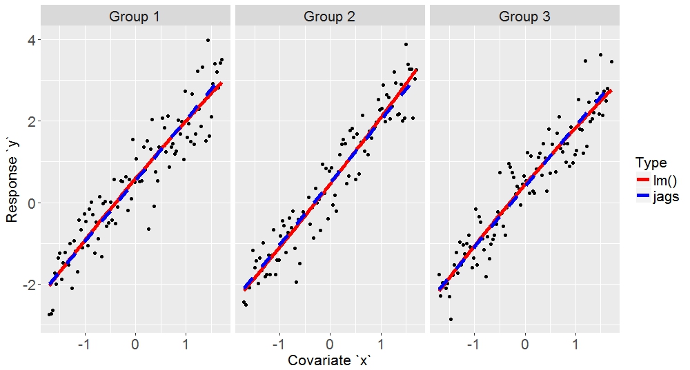
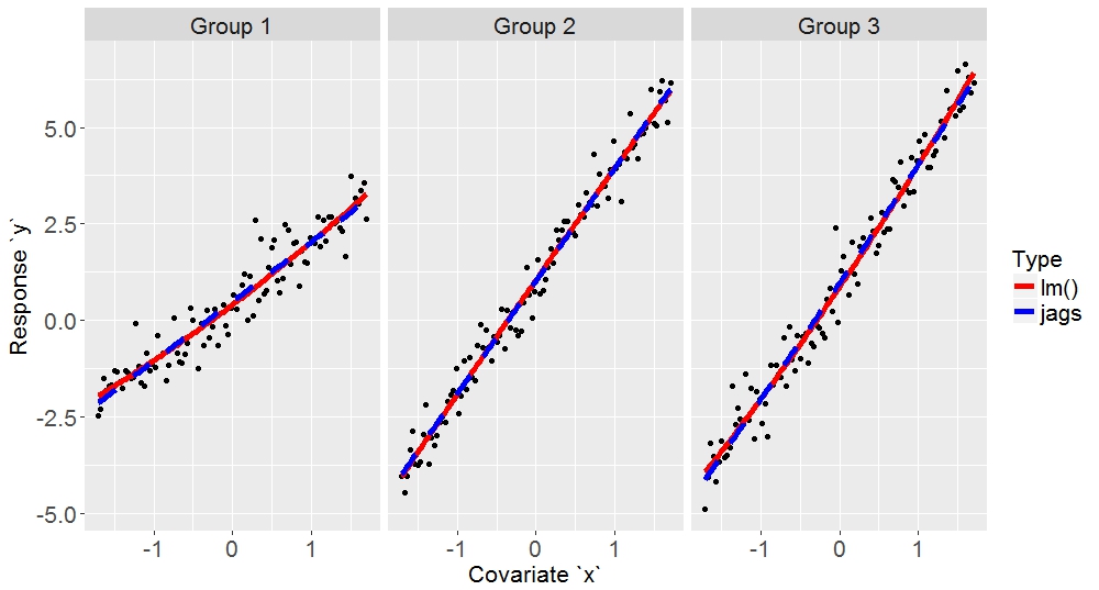
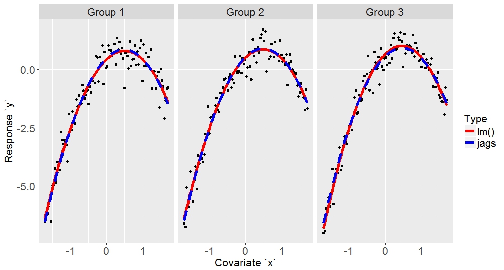
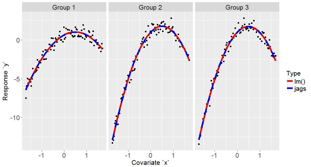
stopCluster(cl)After extensive testing, it seems that the BVS model with backward (for the linear terms) and forward (for the quadratic terms) dependencies returns estimates similar to R’s lm() function, often with better results.
jags estimates:
         a      ag[2]      ag[3]        b1M        b2M     b1Q[2]     b1Q[3]     b2Q[2]
 0.4388473  0.4937112  0.6182427  1.6335965 -1.5419742  1.3599954  1.3835574 -1.3888898
    b2Q[3]      sigma
-1.5621374  0.4846993

lm estimates:
         a      ag[2]      ag[3]        b1M        b2M     b1Q[2]     b1Q[3]     b2Q[2]
 0.4324800  0.5042679  0.6289886  1.6268507 -1.5351445  1.3692690  1.3927054 -1.4003605
    b2Q[3]      sigma
-1.5749945  0.4826420

simulation parameters:
         a      ag[2]      ag[3]        b1M        b2M     b1Q[2]     b1Q[3]     b2Q[2]
 0.4903288  0.5032463  0.4908905  1.5120682 -1.4975522  1.5014423  1.5124471 -1.5010414
    b2Q[3]      sigma
-1.4994300  0.5000000
And the statistical significance of the main effect and interaction terms are:
jags "1 - statistical significance":
iLM iLI iQM iQI
  1   1   1   1
A few more examples
Here are a few typical example fits:
I hope this is helpful to someone.
Please contact me (stephendavidgregory@gmail.com) for more details.
Reuse
Citation
@online{d. gregory2016,
  author = {D. Gregory, Stephen},
  title = {Quadratic Interaction Terms Fitted by {Bayesian} {Variable}
    {Selection}},
  date = {2016-12-21},
  url = {https://stephendavidgregory.github.io/posts/quadratic-interaction-jags},
  langid = {en}
}